31  Using the Tools Together

This unit introduced a framework for determining if there is an association between a quantitative response and a categorical predictor. We formed a standardized statistic for measuring the signal, and developed a model for the data generating process which allowed us to model the null distribution of the standardized statistic. In this chapter, we pull these tools together once more to answer a research question.

The primary question we have been addressing in this unit was whether the moral expectations of students were affected by the type of food to which they were exposed. We saw that there was little evidence of a relationship between these two variables. We now use the data from the Organic Food Case Study to answer a related question:

Do the moral expectations of males and females differ?

Warning

This question enforces a gender binary. Whether the questionnaire provided to students during the study only allowed for “male” and “female,” or whether the responses from participants only included these two genders, we do not know. Those identifying with a gender other than “male” or “female” are not represented by this study, and that is reflected in the above question.

We note that in general, non-binary genders have been historically overlooked in research design.

31.1 Framing the Question (Fundamental Idea I)

As stated, the above question is ill-posed. We have not identified a variable or parameter of interest. We refine this question to be

Does the average moral expectation score of males differ from that of females?

This question could also be stated as the following set of hypotheses:

Let \(\mu_1\) and \(\mu_2\) represent the average moral expectation score for males and females, respectively.
\(H_0: \mu_1 = \mu_2\)
\(H_1: \mu_1 \neq \mu_2\)

31.2 Getting Good Data (Fundamental Idea II)

As we are working with previously collected data, our goal in this discussion is not how best to collect the data but making note of the limitations of the data as a result of how it was collected. We previously described the Organic Food Case Study as an example of a controlled experiment. This was true with regard to the primary question of interest (moral expectations and food exposure). However, the subjects were not randomly assigned to gender; therefore, with regard to this question of interest, the data represents an observational study.

It is common for young researchers to believe that if initially a controlled experiment was performed that the data always permits a causal interpretation. However, we must always examine the data collection with respect to the question of interest. Such “secondary analyses” (using data collected from a study to answer a question for which the data was not initially collected) are generally observational studies. As a result, there may be other factors related to gender and moral expectations that drive any associations we observe.

Warning

When answering a question for which a controlled experiment was not originally designed, carefully consider the question as causal interpretations may no longer be appropriate.

31.3 Presenting the Data (Fundamental Idea III)

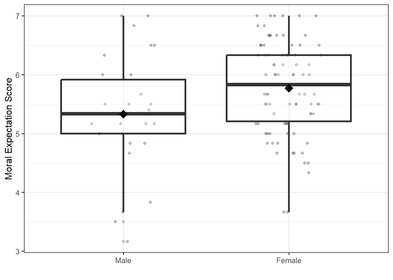
Our question here is examining the relationship between a quantitative response (moral expectation score) and a categorical predictor (gender). Figure 31.1 compares the distribution of the moral expectation score for the two groups. Note that 3 students did not specify their gender; these subjects are removed from the analysis.

Warning

If the group is unknown, the corresponding observation cannot contributed to the analysis. It is therefore common to remove missing values. In this example, however, we note that not specifying a gender may be informative. These individuals may be indicating that they prefer not to provide their gender or that they do not identify with the two gender options available on the questionnaire.

In this case, given the few number of individuals not indicating their gender, we do not feel confident in using their results to make a claim about students who would not provide their gender on such a questionnaire. It is for this reason they were removed from the analysis.

Figure 31.1: Comparison of the moral expectations of males and females. The average value is added for each group. The three students who did not specify their gender are not represented in this graphic.

We note that there were substantially more females in the study than males. This could be a result of the demographics within the home department of the course or demographics of the university at which the study was conducted. From the graphic, it appears the female participants tended to have higher moral expectations by about 1 point, compared to the male participants.

31.4 Quantifying the Variability in the Estimate (Fundamental Idea IV)

In order to measure the size of the signal, we partition the variability in an ANOVA table, which allows us to compute a standardized statistic. In order to partition the variability, we first consider the following model for the data generating process:

\[(\text{Moral Expectation Score})_i = \mu_1(\text{Male})_i + \mu_2 (\text{Female})_i + \varepsilon_i \tag{31.1}\]

where

\[ \begin{aligned} (\text{Male})_i &= \begin{cases} 1 & \text{if i-th participant is male} \\ 0 & \text{otherwise} \end{cases} \\ (\text{Female})_i &= \begin{cases} 1 & \text{if i-th participant is female} \\ 0 & \text{otherwise} \end{cases} \end{aligned} \]

are indicator variables capturing the participant’s gender. Table 31.1 reports the standardized statistic from our study corresponding to testing the hypotheses

\[H_0: \mu_1 = \mu_2 \qquad \text{vs.} \qquad H_1: \mu_1 \neq \mu_2.\]

Table 31.1: ANOVA table summarizing the comparison of the moral expectation score across gender within the Organic Food Case Study.

Term	DF	Sum of Squares	Mean Square	Standardized Statistic
Gender	1	4.363	4.363	6.517
Error	118	79.008	0.670

Of course, if we were to collect a new sample, we would expect our standardized statistic to change. If we want to conduct inference and determine the strength of evidence in this study, we need a model for its null distribution. In order to construct a model for the null distribution of the standardized statistic, we need to place appropriate conditions on the error term. We have three possibilities:

1. The error in the moral expectation score for one individual is independent of the error in the moral expectation score for any other individual.
2. The variance of the error in the moral expectation scores for males is the same as the variance of the error in moral expectation scores for females.
3. The error in the moral expectation score for individuals follows a Normal Distribution.

Before creating a model for the null distribution and computing a p-value, we need to assess whether the data is consistent with these assumptions. This requires examining the residuals from the model. First, we discuss the assumption of independence. Since the data was collected at a single point in time, known as a cross-sectional study, constructing a time-series plot of the residuals would not provide any information regarding this assumption. Instead, we rely on the context of the problem to make some statements regarding whether the data is consistent with this condition (whether making this assumption is reasonable). It is reasonable that the errors are independent. One case in which this might be violated is if students discussed their answers to the questions as they filled out the survey; then, it is plausible that one student influenced another student’s responses. As this is unlikely given the description of the data collection, we feel it is reasonable to assume independence.

Again, note that there is a condition of independence; we are simply saying whether we are willing to assume the condition is satisfied. There is no way to ensure the condition holds.

In order to assess the constant variance condition, let us look back at the boxplots given in Figure 31.1. As the spread of the moral expectation score for each of the two genders is roughly the same, it is reasonable to assume the variability of the errors in each group is the same.

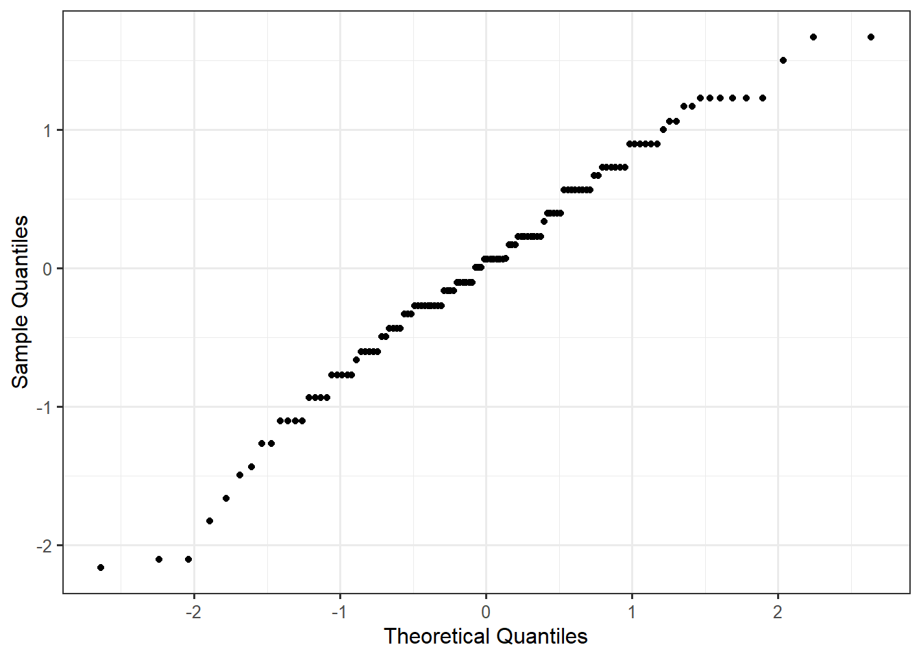
Finally, to assess the Normality condition, we consider a Normal probability plot of the residuals (Figure 31.2). Given that the residuals tend to display a linear relationship, it is reasonable that the errors follow a Normal Distribution.

Figure 31.2: Normal probability plot assessing the assumption that the errors for our model comparing the moral expectation score across gender follow a Normal distribution.

Given that we are comfortable assuming the data is consistent with all conditions from the classical ANOVA model (Definition 28.1), we can make use of an analytical model for the null distribution.

31.5 Quantifying the Evidence (Fundamental Idea V)

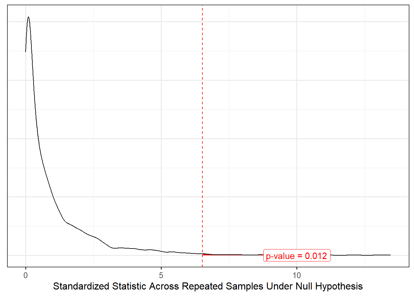
Now that we have a model for the null distribution of our standardized statistic, we can determine how extreme our particular sample was by comparing the standardized statistic for our sample with this null distribution (Figure 31.3).

Figure 31.3: Analytical model of the null distribution of the standardized statistic computed from the Organic Foods Case Study comparing the moral expectation scores across males and females.

Based on the results, the study suggests there is some evidence (p = 0.012) that the average moral expectations of male students differs from that of female students. Looking back at Figure 31.1, females tend to have higher moral expectations on average.

31.6 Conclusion

Throughout this unit, we have examined a framework for examining the association between a quantitative response and a categorical predictor. This reinforces a couple of big ideas we have seen throughout this text:

• The key to measuring a signal is to partition the variability in the response.
• A standardized statistic is a numeric measure of the signal strength in the sample.
• Modeling the data generating process provides us a way of modeling the sampling distribution of the parameter estimates and the null distribution of a standardized statistic when combined with conditions on the stochastic portion of the model for the data generating process.
• Before imposing conditions on the stochastic portion of a data generating process, we should graphically assess whether the data is consistent with these conditions.