39 Assessing the Modeling Conditions in Repeated Measures ANOVA
In this unit we have discussed a model relating a quantitative response to a categorical predictor in the presence of blocks that induce correlation among the responses. For the Frozen Yogurt Case Study, our model had the form
\[ \begin{aligned} (\text{Taste Rating})_i &= \theta_1 (\text{East Side})_i + \theta_2 (\text{Name Brand})_i + \theta_3 (\text{South Side})_i \\ &\qquad + \beta_2 (\text{Participant 2})_i + \beta_3 (\text{Participant 3})_i + \beta_4 (\text{Participant 4})_i \\ &\qquad + \beta_5 (\text{Participant 5})_i + \beta_6 (\text{Participant 6})_i + \beta_7 (\text{Participant 7})_i \\ &\qquad + \beta_8 (\text{Participant 8})_i + \beta_9 (\text{Participant 9})_i + \varepsilon_i \end{aligned} \]
where we use the same indicator variables defined in Chapter 36. Further, we considered several conditions on the distribution of the error term and the distribution of the block effects:
- The error in the taste ratings within one individual is independent of the error in the taste ratings within any other individual.
- The variability in the error in the taste ratings is the same for all vendor and participant combinations.
- The error in the taste ratings follows a Normal distribution.
- The deterministic portion of the model is correctly specified; that is, any differences in the average ratings across vendors is the same for all participants.
- One participant’s preferences relative to the population is independent of any other participant’s preferences; that is, the block effects are independent of one another.
- Each participant’s preferences relative to the population is independent of of the error in the taste ratings of all individuals; that is, the block effects are independent of the error terms.
- Participants’ preferences follow a Normal distribution; that is, the block effects follow a Normal distribution.
While we imposed each of these conditions in Chapter 38, we could have developed an empirical model for the null distribution of the standardized statistic imposing only a subset of these conditions. Unfortunately, we cannot simply state conditions and then proceed blindly. In order to rely on the p-values and confidence intervals produced from any modeling procedure, the data must be consistent with the conditions imposed.
In this section, we discuss how we assess these conditions qualitatively. We note that the last three conditions on the block effects are not easily assessed. These are generally stated and assumed.
The conditions on the block effects in a repeated measures ANOVA model are not easily assessed and tend to be stated and assumed in practice.
Just as we saw in Chapter 20 and Chapter 30, however, the first four conditions placed on the error distribution can be assessed using residuals.
39.1 Residual
The difference between the observed response and the predicted response (estimated deterministic portion of the model). Specifically, the residual for the \(i\)-th observation is given by
\[(\text{Residual})_i = (\text{Response})_i - (\text{Predicted Mean Response})_i\]
where the “predicted mean response” is often called the predicted, or fitted, value.
Residuals mimic the noise in the data-generating process.
For the repeated measures ANOVA model, the predicted mean response is determined by using the least squares estimates from the model:
\[(\text{Predicted Mean Response})_i = \sum_{j=1}^{k} \widehat{\theta}_j (\text{Group } j)_i + \sum_{m=2}^{b} \widehat{\beta}_m (\text{Block } m)_i.\]
The conditions are placed on the error term, but they are assessed with residuals.
39.2 Assessing the Independence Condition
The error in the taste ratings within one individual is independent of the error in the taste ratings within any other individual.
Generally, independence is assessed by considering the method in which the data was collected and considering the context with a discipline expert. By carefully considering the manner in which the data was collected, we can typically determine whether it is reasonable that the errors in the response are independent of one another. When a study design incorporates blocking, it was because researchers had identified a source of correlation prior to conducting the study. Further, the researchers are generally willing to assume that observations within the block are independent of one another and the units in different blocks are independent of one another. That is, the study design considered the possible sources of correlation and accounted for them by noting the blocks and then using those blocks in the model for the data-generating process.
While the incorporation of the blocks into the model for the data-generating process should eliminate any correlation in the errors due to observations being from the same block, it is possible that other forms of correlation exist. For example, if the data is collected over time, it is possible that observations collected in proximity to one another exhibit a relationship; and, such a relationship would not be captured by the block terms. When we know the order in which the data was collected, we can assess whether the data tends to deviate from the condition of independence over time. This is done graphically through a time-series plot of the residuals. If the errors are unrelated, then the value of one residual should tell us nothing about the value of the next residual. Therefore, a plot of the residuals over time should look like noise (since residuals are supposed to mimic the noise in the model). If there are any trends, then it suggests the data is not consistent with independence.
39.3 Time-Series Plot
A time-series plot of a variable is a line plot with the variable on the y-axis and time on the x-axis.
If the data is consistent with the independence condition, we would not expect to see a trend in the location or spread in a time-series plot of the residuals. Note that this graphic can only be used if the order in which the data was collected is known, and the order indicates some natural timing. Otherwise, we generally assume the inclusion of the block terms captured the primary source of correlation among responses.
For the Frozen Yogurt Case Study, participants were assessed simultaneously within the class. Therefore, there is no ordering in time to be concerned about. As such, a time-series plot of the residuals would not be useful here. Considering the context, the students were the ones who had designed the study (it was carried out by their instructor); therefore, they prioritized the quality of the data collection. The students did their best to not influence the ratings of any other participant. It is reasonable to assume the data is consistent with the independence condition once the repeated measures have been accounted for by the inclusion of the block terms in the model.
39.4 Assessing Homoskedasticity
The variability in the error in the taste ratings is the same for all vendor and participant combinations.
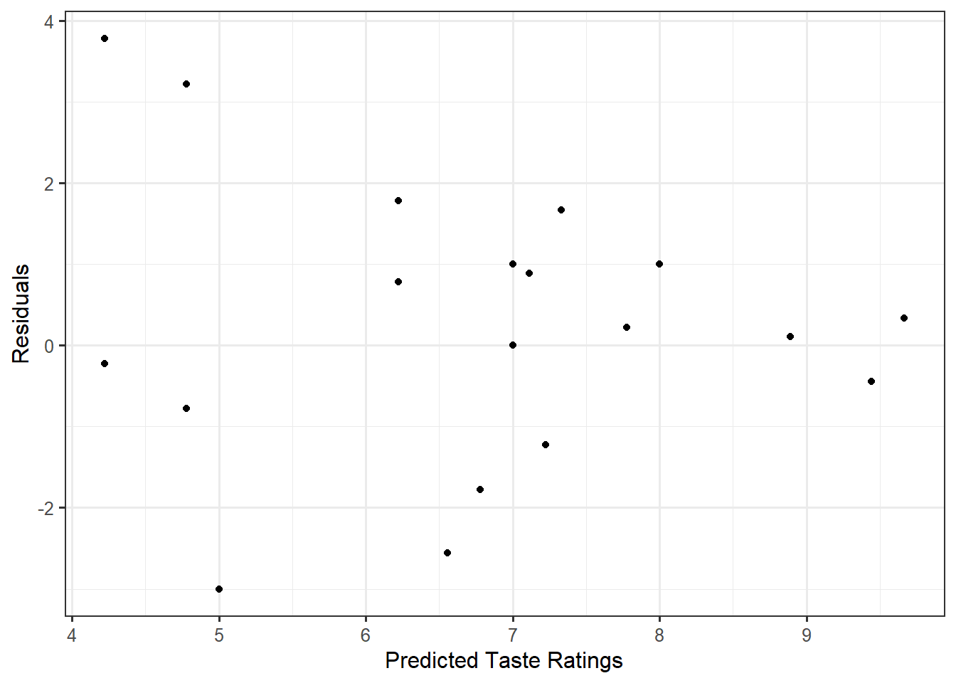
We want the variability of the errors to be the same across all values of the predictors — that is what is being captured with the phrase “all vendor and participant combinations.” As a result, unlike Chapter 30, we cannot simply make a boxplot of the residuals across the three vendors. Once there is more than one variable in the deterministic portion of the model for the data-generating process, we must resort back to the strategy discussed in Chapter 20. That is, we construct a plot of the residuals against the predicted values.
Even though our goal is to compare the mean response across groups as in ANOVA, since a repeated measures ANOVA model contains multiple variables in the deterministic portion of the model for the data-generating process, we cannot assess the constant variance condition in the same way.
If the data is consistent with the constant variance condition, there should be no trends in the spread of the residuals when plotted against the predicted mean response (the fitted values).
Figure 39.1 shows the residuals for each individual across the predicted taste rating for that individual observation. Notice that as the predicted taste ratings increase, the variability in the residuals tends to decrease. This is inconsistent with what we would expect if the variability in the errors was constant. That is, if the variability of the errors was constant, we would not expect the spread of the residuals to exhibit this “fan” shape. Therefore, we do not feel it is reasonable to impose the constant variance condition.

39.5 Assessing Normality
The error in the taste ratings follows a Normal distribution.
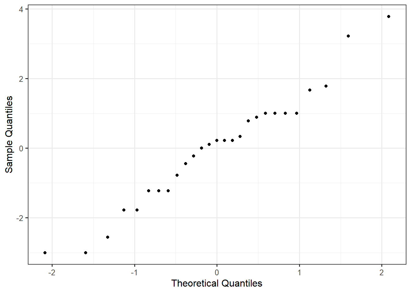
If the errors follow a Normal distribution, then we would expect the residuals to mimic a sample taken from a Normal distribution. As introduced in Chapter 20, we emphasize the Normal probability plot for assessing the Normality condition.
39.6 Probability Plot
Also called a “Quantile-Quantile Plot”, a probability plot is a graphic for comparing the distribution of an observed sample with a theoretical probability model for the distribution of the underlying population. The quantiles observed in the sample are plotted against those expected under the theoretical model.
If the data is consistent with the normality condition, the Normal probability plot of the residuals should exhibit a straight line with any deviations appearing to be random. Systemic deviations from a straight line indicate the observed distribution does not align with the proposed model.
Figure 39.2 shows the probability plot for the residuals from the Frozen Yogurt Case Study.

Overall, the points do tend to follow a straight line. It seems reasonable the data is consistent with the errors following a Normal distribution.
Keep in mind the probability plot of the residuals can only be used to assess the condition placed on the error term. This cannot be used to make a statement about the condition placed on the block effects.
39.7 Assessing Whether the Model is Correctly Specified
The deterministic portion of the model is correctly specified; that is, any differences in the ratings across vendors is the same for all participants.
Recall that the structure of our repeated measures ANOVA model suggests that any differences in the average response between groups are the same across all blocks. This is analogous to assuming a specific functional form for the relationship between two predictors (for example, linear or sinusoidal). Because we are discussing the structure of the deterministic portion of the model for the data-generating process, occasionally, we can assess this condition from the context of the problem with the help of a discipline expert. For example, do we believe it is reasonable to believe that every individual will have the same vendor preference for frozen yogurt? Our personal experience alone tells us one person’s favorite restaurant is not necessarily everyone’s favorite restaurant; so, there is some reason already to doubt this condition is reasonable for the Frozen Yogurt Case Study.
When we (or the discipline experts) do not have enough knowledge to confidently assess this condition, we can examine a graphic of the residuals and predicted values. Recall that in Chapter 18 and Chapter 20, we argued that the deterministic portion of the model being correctly specified was the result of the errors having a value of 0, on average. That is, the mean-0 condition is synonymous with requiring the deterministic portion of the model for the data-generating process to have the correctly specified structure.
If the errors have a mean of 0 for all combination of variables in the deterministic portion of the model, then we would expect the residuals to have a mean of 0 for all predicted values. That is, if the data is consistent with the mean-0 condition, then as we move left to right across a plot of the residuals and predicted values, the residuals should tend to balance out at 0 everywhere along the x-axis. Any trends in the location of this graphic would indicate the data is not consistent with the mean-0 condition.
If the data is consistent with the mean-0 condition, there should be no trends in the location of the plot of the residuals when plotted against the predicted values.
As we examine Figure 39.1, the residuals do tend to balance out at 0 everywhere along the x-axis. That is, we do not see a trend in the location of the residuals as the predicted values increase. Therefore, it is reasonable to say the sample is consistent with the mean-0 condition.
The sample seems to be at odds with our personal experience. Remember, we cannot use the graphic to confirm the condition is met; we can only say the data is consistent with the behavior we would expect of the residuals if the the condition were true. It is probably the case that any differences in vendor preferences across individuals is so slight that the structure we have imposed is reasonable in this sample.
39.8 General Tips for Assessing Assumptions
First discussed in Chapter 20, we want to remember four things that should be kept in mind when assessing conditions:
- We should not spend an extraordinary amount of time examining any one residual plot; we might convince ourselves of patterns that do not exist. We are looking for major deviations from our expectations.
- We can never prove a condition is satisfied; we can only determine whether the data is consistent with a condition or whether it is not consistent with a condition.
- Any condition required for a particular analysis should be assessed.
- Transparency is crucial.
In this chapter, we add to these four tips that conditions placed on the block effects cannot be graphically assessed.